Hackathon - Benjamin Blodgett Wyatt Radkiewicz
23 April 2025

Background
It took us a bit of time to figure out what is going on statistically. Basically we are looking at the difference between two players or teams and their respective “elo” or performance ranking. We can then plug the horizontal difference between the elo distribution of the two players or teams into a sigmoid equation to attempt to predict success of one team or player winning over the other. This sigmoid equation ranges between 0 and 1 because probability can’t exceed 100% or go under 0%. Our k value in the code represents the volatility of the added rating. A low k means the results of the event will have a low impact on the win success rating.
Improving the Model
First lets try to only use the later half of the games in the season for our model. We did this by changing the range of the games for loop. We divide the range by two and offset by half to get the most recent half of games.
Initial Results
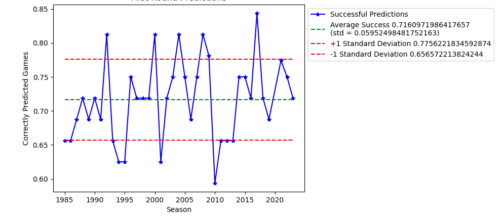
We look at the average success rate and standard deviation of our prediction.
| % | σ | |
|---|---|---|
| Starting Values | 0.7078 | 0.0569 |
| Excluding Early Half | 0.6008 | 0.0809 |
Where % is the average success rate and σ is the standard deviation.
Rivalry Scoring
One idea we had was trying to determine whether two teams have a rivalry. If they are rivals, we can increase the k value correspondingly and increase the effect of the results on the rating. As you can see, this marginally increased our success rate of predictions, but at the cost of increasing the standard deviation.
| % | σ | |
|---|---|---|
| Starting Values | 0.7078 | 0.0569 |
| Excluding Early Half | 0.6008 | 0.0809 |
| Rivalry Scoring (decay) | 0.7120 | 0.0590 |
We achieved this result with exponential decay. Repeated success one way or the other would decrease the rivalry amount.
Parity Scoring
Our next idea was to simply look at the all time victory and successes between two teams. If they had a more equal amount of wins and losses against each other then we consider them to be rivals. Alternatively, if their chance of success over time is more disproportionate, we do not consider them rivals, and hence the k value will be lower.
| % | σ | |
|---|---|---|
| Starting Values | 0.7078 | 0.0569 |
| Excluding Early Half | 0.6008 | 0.0809 |
| Rivalry Scoring (decay) | 0.7120 | 0.0590 |
| Parity Scoring | 0.7111 | 0.0624 |
This was perhaps because we weighted “closeness” too heavily. After adjusting the effect we were able to achieve our highest yet success rate with a standard deviation only marginally higher than baseline.
| % | σ | |
|---|---|---|
| Starting Values | 0.7078 | 0.0569 |
| Excluding Early Half | 0.6008 | 0.0809 |
| Rivalry Scoring (decay) | 0.7120 | 0.0590 |
| Parity Scoring | 0.7111 | 0.0624 |
| Parity Scoring (light) | 0.7128 | 0.0579 |
Previously we look at the relationship between pairs of teams and their history. Next we want to determine what makes individual teams special. We do this by trying to find which teams are erratic in performance, and which are consistent. For teams we deem erratic, we increase the k value.
| % | σ | |
|---|---|---|
| Starting Values | 0.7078 | 0.0569 |
| Excluding Early Half | 0.6008 | 0.0809 |
| Rivalry Scoring (decay) | 0.7120 | 0.0590 |
| Parity Scoring | 0.7111 | 0.0624 |
| Parity Scoring (light) | 0.7128 | 0.0579 |
| Erratic Scoring | 0.7153 | 0.0630 |
We were unsure whether or not this made sense. If a team is incredibly consistent in wins or losses then a single data point to the contrary shouldn’t necessarily be weighted more heavily. It could be an outlier or indicate a temporary change in the roster of the team. Maybe a specific key player is performing above usual expectations, but rosters change with time, and high performing players may move on to greater opportunities on other teams or even outside of sports. What we really want to identify are the underlying factors which make a specific team successful or not over the long run. Thusly, we will next attempt to weight consistency with a higher k and a greater impact on the scoring.
| % | σ | |
|---|---|---|
| Starting Values | 0.7078 | 0.0569 |
| Excluding Early Half | 0.6008 | 0.0809 |
| Rivalry Scoring (decay) | 0.7120 | 0.0590 |
| Parity Scoring | 0.7111 | 0.0624 |
| Parity Scoring (light) | 0.7128 | 0.0579 |
| Erratic Scoring | 0.7153 | 0.0630 |
| Erratic Scoring (inverse)1 | 0.714 | 0.064 |
The data appear to fit our original hypothesis better. We must weight the k higher in cases where a team’s performance is erratic. Perhaps because it is an indication that the trend is changing. If this is occurring then more emphasis should be placed on newer results in order to replace the old status quo somewhat.
More experimenting with the parameters of the standard erratic scoring give us a better result.
| % | σ | |
|---|---|---|
| Starting Values | 0.7078 | 0.0569 |
| Excluding Early Half | 0.6008 | 0.0809 |
| Rivalry Scoring (decay) | 0.7120 | 0.0590 |
| Parity Scoring | 0.7111 | 0.0624 |
| Parity Scoring (light) | 0.7128 | 0.0579 |
| Erratic Scoring | 0.7153 | 0.0630 |
| Erratic Scoring (inverse) | 0.7140 | 0.0640 |
| Erratic Scoring (improved) | 0.7160 | 0.060 |
Next we try to determine whether or not one team is more or less tired than the other, and subtract elo slightly from the tired team. Our method is to see whether the last game played from the team was less than 3 days ago. If so, we subtract 30 points from that team’s elo rating.
| % | σ | |
|---|---|---|
| Starting Values | 0.7078 | 0.0569 |
| Excluding Early Half | 0.6008 | 0.0809 |
| Rivalry Scoring (decay) | 0.7120 | 0.0590 |
| Parity Scoring | 0.7111 | 0.0624 |
| Parity Scoring (light) | 0.7128 | 0.0579 |
| Erratic Scoring | 0.7153 | 0.0630 |
| Erratic Scoring (inverse) | 0.7140 | 0.0640 |
| Erratic Scoring (improved) | 0.7160 | 0.0600 |
| Exhaustion Scoring | 0.7103 | 0.0544 |
Our query was especially slow. Exhaustion scoring also didn’t improve our results. This is our last attempt to improve our prediction. Next time we will consider using a different language or set of tools. Here is the link to the Jupyter notebook. Our work was done in the very bottom snippet of code.
- by “(inverse)” here we mean that consistency implies higher k